Improved EMA & CDC Trailing Stop StrategyImproved EMA & CDC Trailing Stop Strategy
Objective: This strategy seeks to exploit potential trend reversals or continuations using Exponential Moving Averages (EMAs) and a trailing stop based on the Chande Dynamic Convergence Divergence (CDC) ATR method.
Components:
Exponential Moving Averages (EMAs):
60-period EMA (Blue Line): Faster-moving average that reacts more quickly to price changes.
90-period EMA (Red Line): Slower-moving average that provides a smoother indication of long-term price direction.
MACD Indicator:
Utilized to confirm the trend direction. When the MACD line is above its signal line, it may indicate a bullish trend. Conversely, when the MACD line is below its signal line, it may indicate a bearish trend.
CDC Trailing Stop ATR:
Used to set dynamic stop-loss levels that adjust with market volatility. This stop is based on the Average True Range (ATR) with a user-defined multiplier, providing the strategy with a flexible way to protect against adverse price movements.
Profit Targets:
Based on a multiple of the ATR, this sets an objective level at which to take profits, ensuring gains are captured while potentially still leaving room for further profitable movement.
Trading Rules:
Entry:
Long (Buy) Entry Conditions:
Price is above the 60-period EMA.
The 60-period EMA is above the 90-period EMA.
The MACD line is above its signal line.
Price is above the calculated CDC Trailing Stop ATR level.
Short (Sell) Entry Conditions:
Price is below the 60-period EMA.
The 60-period EMA is below the 90-period EMA.
The MACD line is below its signal line.
Price is below the calculated CDC Trailing Stop ATR level.
Exit:
Long (Buy) Exit Conditions:
Price reaches the predetermined profit target based on the ATR.
Price drops below the CDC Trailing Stop ATR level.
Short (Sell) Exit Conditions:
Price reaches the predetermined profit target based on the ATR.
Price rises above the CDC Trailing Stop ATR level.
Visualization:
The strategy displays the 60-period and 90-period EMAs on the chart.
The CDC Trailing Stop ATR levels for both long and short trades are also plotted for clarity.
The MACD Histogram is shown to visualize the difference between the MACD line and its signal line.
Recommendations: Before deploying this strategy, traders should backtest it across various historical data sets and market conditions. Regularly reviewing and potentially adjusting the strategy is recommended as market dynamics evolve.
Cari dalam skrip untuk "take profit"

Buy/Sell BoxThis indicator tries to identify the points where the price exceeds or falls below a rectangle based on the opening and closing prices of the previous period, the creation of the boxes occurs when a doji is detected therefore it will calculate the coordinates of the rectangle that will be drawn around it, therefore the indicator offers buy or sell signals based on this logic. Specifically, the buy signal is generated if the closing price is above the top of the rectangle and satisfies some previous price conditions while the sell signal is generated if the closing price is below the bottom of the rectangle and satisfies some conditions of previous prices within a further threshold based on the Ema 150.
Lines are then drawn on the graph to visually display the extreme price levels, which can be useful for any confirmation of buy and sell signals, Stop Loss and Take Profit, Trend Filter (to visually understand if the trend is bullish or bearish)
A potentially effective trading strategy could involve identifying buy and sell signals near the extreme price level lines drawn by the indicator. This approach can be used to try to improve the accuracy of your trading signals and make more informed decisions. For example:
When you receive a buy or sell signal based on the dojis and rectangles generated by the indicator, check whether the price is also near one of the extreme price level lines. If you are receiving a buy signal and notice that the current price is near a low of the lower level line, this may further confirm the buying opportunity, as the price is near a significant resistance level. On the contrary, if the sell signal was close to a maximum price level it could confirm an excellent short entry.
It is also possible to use the boxes as reference points to set the stop loss and take profit levels. If you are entering a buy position, you might consider setting your stop loss just below an upper line of the last box. Additionally, you may want to set your take profit near a higher price level if you are looking to maximize profits. This will help manage risks and protect your capital.

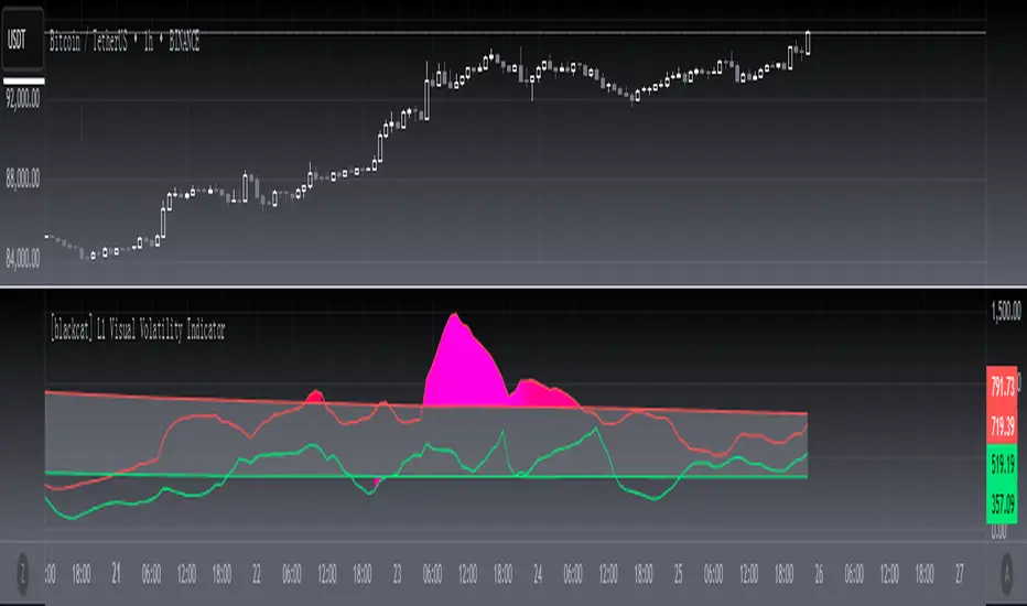
[blackcat] L1 Visual Volatility IndicatorHey there! Let's get into the details about dynamic rate indicators, how they work, their importance, usage, and benefits in trading.
Dynamic rate indicators are essential in trading as they help traders assess the volatility and risk level of the market, so they can make the right trading strategies and risk management measures.
When it comes to the importance of dynamic rate indicators, they provide critical information about market volatility, which is super important for traders. Traders can use this information to understand the risk level of the market, determine market stability and instability, and adjust trading strategies based on volatility changes.
Now let's talk about the usage of dynamic rate indicators. They have different usage times for different trading strategies and market environments. Generally, when market volatility is low, traders can take advantage of the opportunity to do trend tracking or oscillating trades. When market volatility is high, traders can take a more conservative approach, such as using stop-loss orders or reducing position sizes.
Using dynamic rate indicators can bring several benefits. First, they can help traders evaluate the risk level of the market, so they can develop suitable risk management strategies. Traders can adjust stop-loss and take-profit levels based on changes in volatility to control risk. Second, dynamic rate indicators provide information about market trends and price fluctuations, helping traders make wiser trading decisions. Traders can determine entry and exit points based on the signals of dynamic rate indicators. Lastly, dynamic rate indicators play a significant role in option pricing. Implied volatility helps traders evaluate option prices and market expectations for future volatility, so they can carry out option trades or hedging operations.
In conclusion, dynamic rate indicators are essential for traders as they help assess market volatility and risk levels, develop suitable trading strategies and risk management measures, and increase trading success and profitability. Remember that different indicators are suitable for different types of markets, so it is essential to choose the right one for your specific trading needs.
This indicator is a powerful tool for traders who want to stay ahead of the market and make informed trading decisions. By analyzing trends in volatility, this indicator can provide valuable insights into market sentiment and help traders identify potential trading opportunities.
One of the key advantages of the L1 Visual Volatility Indicator is its ability to adapt to changing market conditions. The channel structure it constructs based on ATR characteristics provides a framework for tracking volatility that can be adjusted to different timeframes and asset classes. This allows traders to customize the indicator to their specific needs and trading style, making it a versatile tool for a wide range of trading strategies.
Another advantage of this indicator is its use of gradient colors to differentiate between Bullish and Bearish volatility. This provides a visual representation of market sentiment that can help traders quickly identify potential trading opportunities and make informed decisions. Additionally, the use of Fibonacci's long-term moving average to define the sideways consolidation area provides a reliable framework for identifying key levels of support and resistance, further enhancing the indicator's usefulness in trading.
In conclusion, the L1 Visual Volatility Indicator is a powerful tool for traders looking to stay ahead of the market and make informed trading decisions. Its ability to adapt to changing market conditions and use of gradient colors to differentiate between Bullish and Bearish volatility make it a versatile and effective tool for a wide range of trading strategies. By incorporating this indicator into their trading arsenal, traders can gain valuable insights into market sentiment and improve their chances of success in the markets.
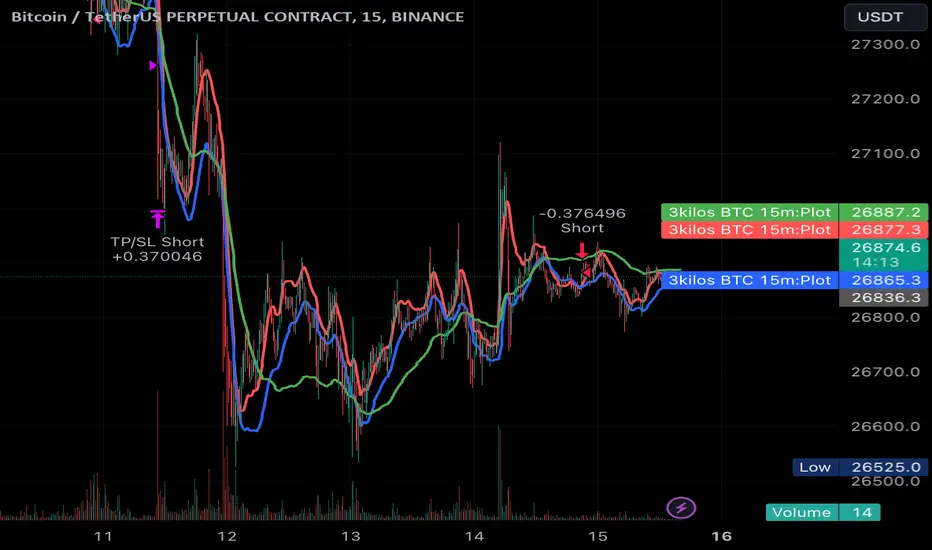
3kilos BTC 15mThe "3kilos BTC 15m" is a comprehensive trading strategy designed to work on a 15-minute timeframe for Bitcoin (BTC) or other cryptocurrencies. This strategy combines multiple indicators, including Triple Exponential Moving Averages (TEMA), Average True Range (ATR), and Heikin-Ashi candlesticks, to generate buy and sell signals. It also incorporates risk management features like take profit and stop loss.
Indicators
Triple Exponential Moving Averages (TEMA): Three TEMA lines are used with different lengths and sources:
Short TEMA (Red) based on highs
Long TEMA 1 (Blue) based on lows
Long TEMA 2 (Green) based on closing prices
Average True Range (ATR): Custom ATR calculation with EMA smoothing is used for volatility measurement.
Supertrend: Calculated using ATR and a multiplier to determine the trend direction.
Simple Moving Average (SMA): Applied to the short TEMA to smooth out its values.
Heikin-Ashi Close: Used for additional trend confirmation.
Entry & Exit Conditions
Long Entry: Triggered when the short TEMA is above both long TEMA lines, the Supertrend is bullish, the short TEMA is above its SMA, and the Heikin-Ashi close is higher than the previous close.
Short Entry: Triggered when the short TEMA is below both long TEMA lines, the Supertrend is bearish, the short TEMA is below its SMA, and the Heikin-Ashi close is lower than the previous close.
Take Profit and Stop Loss: Both are calculated as a percentage of the entry price, and they are set for both long and short positions.
Risk Management
Take Profit: Set at 1% above the entry price for long positions and 1% below for short positions.
Stop Loss: Set at 3% below the entry price for long positions and 3% above for short positions.
Commission and Pyramiding
Commission: A 0.07% commission is accounted for in the strategy.
Pyramiding: The strategy does not allow pyramiding.
Note
This strategy is designed for educational purposes and should not be considered as financial advice. Always do your own research and consider consulting a financial advisor before engaging in trading.
Based RSI (BullDozz)Installation: To use this script, open TradingView and create a new Pine Script strategy. You can paste the code provided into the Pine Script editor.
Customizable Inputs: The script includes various input parameters that you can customize to fit your trading preferences. These parameters are defined using the input function and include values like length, TPPercent, and others. You can adjust these values based on your trading strategy.
Strategy Signals: The script generates buy and sell signals based on the conditions specified in the buySignal and sellSignal variables. These signals are derived from the analysis of the oscillator (osc) and the Relative Strength Index (rsi). When a buy signal occurs, the script enters a long position, and when a sell signal occurs, it enters a short position.
Take Profit: The script includes a take profit feature (useTP) that allows you to enable or disable take profit orders. When enabled, it calculates take profit levels based on the specified percent (TPPercent) and attaches them to the open positions.
Plotting: The script also visualizes the oscillator (osc) and a midline (0) on the chart using histogram-style bars. The colors of these bars change based on the oscillator's direction.

Position and Risk Calculator (for Indices) [dR-Algo]Position and Risk Calculator : Your Ultimate Risk Management Tool for Indices
The difference between a novice and a seasoned trader often comes down to one essential element: risk management. While trading indices, the challenges are even more intense due to market volatility and leverage. The Position and Risk Calculator steps in here to bridge the gap, providing you with an efficient tool designed exclusively for indices trading.
Key Features:
User-Friendly Interface: Designed to integrate effortlessly with your TradingView chart, this tool's interface is intuitive and clutter-free.
Dynamic Price Level Adjustment: Move your Entry, Stop Loss, and Take Profit levels directly on the chart for an interactive experience.
Account Balance Input: Customize the tool to understand your unique financial situation by inputting your current account balance.
Trade Risk Customization: Define how much you're willing to risk per trade, and the tool will do the rest.
Automated Calculations: The indicator calculates the maximum monetary risk and translates it into the maximum lot size you can afford. It delivers a full-integer lot size to make your trading decisions easier.
Comprehensive Risk Evaluation: Beyond lot sizes, it provides you with the Cost-to-Reward Ratio (CRV) of your trade, the actual monetary risk according to the calculated lot size, and the potential profit.
How To Use:
Once you add the Position and Risk Calculator to your TradingView chart, a new interactive panel appears. Here’s how it works:
Set Price Levels: Using draggable lines on the chart, set your Entry Price, Stop Loss, and Take Profit levels.
Account Details: Go to settings and enter your Account Balance and your desired risk percentage per trade.
Automatic Calculations: As soon as the above details are set, the indicator goes to work. It first calculates your maximum risk in monetary terms and then translates that into the maximum lot size you can take for the trade.
Review and Trade: The indicator shows you all the vital statistics - CRV of the trade, the money at risk according to the calculated lot size, and the possible profit.
Why Choose This Tool?
Informed Decisions: Your trading decisions will be based on concrete numbers, removing guesswork.
Time-saving: No need for manual calculations or using separate tools; everything is in one place.
Focus on Trading: By automating the risk management aspect, this tool allows you to focus more on your trading strategy and market analysis.
Tailor-Made for Indices: Unlike many other tools that try to serve all markets, the Position and Risk Calculator is designed specifically for indices trading.
Remember, effective risk management is what separates successful traders from those who burn out. The Position and Risk Calculator not only helps you define your risk but also helps you understand it, empowering you to trade with confidence.
So why not give yourself the best chance of success? Add the Position and Risk Calculator to your TradingView setup and experience the difference it can make.

Trend Analyser by Abdul KhaderThis indicator is designed to provide buy and sell signals based on a combination of technical analysis methods. It uses the Relative Strength Index (RSI), Moving Average Convergence Divergence (MACD), and Exponential Moving Averages (EMA) to generate signals. It also calculates Stop Loss (SL) and Take Profit (TP) levels based on the Average True Range (ATR).
Components:
RSI: An oscillator that measures the speed and change of price movements. RSI is used to identify overbought and oversold conditions. In this indicator, an RSI below 30 is considered oversold and an RSI above 70 is considered overbought.
MACD: A trend-following momentum indicator that shows the relationship between two moving averages of a security’s price. The MACD triggers technical signals when it crosses above (to buy) or below (to sell) its signal line.
EMA: These moving averages give more weight to recent prices and are used to identify short-term price trends. A crossover of a shorter period EMA (9 periods in this case) above a longer period EMA (21 periods in this case) generates a buy signal. Conversely, a crossover of the shorter EMA below the longer EMA generates a sell signal.
ATR: This is a market volatility indicator. The ATR is used to calculate Stop Loss and Take Profit levels. These levels are set at a distance from the entry price, equal to a certain multiplier (1.5 in this case) of the ATR.
How to Use:
Buy Signal: A green triangle below the price bar indicates a buy signal. This is generated when the following conditions are met:
The short-term EMA crosses above the long-term EMA
The RSI is below 30 (oversold condition)
The MACD line crosses above the signal line and is above zero
Sell Signal: A red triangle above the price bar indicates a sell signal. This is generated when the following conditions are met:
The short-term EMA crosses below the long-term EMA
The RSI is above 70 (overbought condition)
The MACD line crosses below the signal line and is below zero
Stop Loss and Take Profit: These levels are indicated by dashed lines. The stop loss for a long position is set below the entry price, while the take profit is set above. For a short position, the stop loss is set above the entry price and the take profit is set below.
Important Notes:
This indicator is designed for intraday trading and may not be suitable for longer-term trades.
Always use this indicator in conjunction with other aspects of technical and fundamental analysis. No indicator can provide accurate signals 100% of the time.
Always backtest this indicator with historical data before using it in live trading.
Risk management is crucial in trading. Never risk more than a small percentage of your trading capital on a single trade.
CC Trend strategy 2- Downtrend ShortTrend Strategy #2
Indicators:
1. EMA(s)
2. Fibonacci retracement with a mutable lookback period
Strategy:
1. Short Only
2. No preset Stop Loss/Take Profit
3. 0.01% commission
4. When in a profit and a closure above the 200ema, the position takes a profit.
5. The position is stopped When a closure over the (0.764) Fibonacci ratio occurs.
* NO IMMEDIATE RE-ENTRIES EVER!*
How to use it and what makes it unique:
This strategy will enter often and stop quickly. The goal with this strategy is to take losses often but catch the big move to the downside when it occurs through the Silvercross/Fibonacci combination. This is a unique strategy because it uses a programmed Fibonacci ratio that can be used within the strategy and on any program. You can manipulate the stats by changing the lookback period of the Fibonacci retracement and looking at different assets/timeframes.
This description tells the indicators combined to create a new strategy, with commissions and take profit/stop loss conditions included, and the process of strategy execution with a description of how to use it. If you have any questions feel free to PM me and boost if you found it helpful. Thank you, pineUSERS!
CHEATCODE1

Impulse MACD buy OwlPixelDescription:
The Impulse MACD Buy Indicator, developed by OwlPixel, is a powerful trading tool for traders using TradingView's Pine Script version 5. This indicator aims to provide valuable insights for identifying potential buy signals in the market using the popular MACD (Moving Average Convergence Divergence) oscillator.
Key Features:
MACD Analysis: The indicator displays the MACD line (blue) and the signal line (orange) on the chart, helping traders assess the momentum and trend direction of an asset.
Impulse Histo: The Impulse Histo (blue histogram) visualizes the difference between the MACD line and the signal line, making it easier to spot changes in market strength and potential trend reversals.
Impulse MACD CD Signal: This histogram (maroon color) highlights the divergence between the Impulse Histo and the signal line, providing further insights into trend shifts.
Background Boxes: The indicator features three rows of different colored background boxes that represent distinct market conditions - an uptrend (light green), a downtrend (light red), and a neutral trend (light yellow).
Crossover Points: Buy signals are marked with green circles when the MACD line crosses above the signal line, suggesting potential entry points for long positions.
Demand and Supply Bars: The demand (lime/green) and supply (red/orange) bars are intensified, aiding traders in identifying possible reversal areas.
Stop Loss and Take Profit:
The Impulse MACD Buy Indicator automatically calculates Stop Loss (SL) and Take Profit (TP) levels for buy signals. The SL level is set at the highest of the last three candles, while the TP level is determined by a user-defined percentage of the closing price. This information helps traders manage risk and optimize their profit potential.
Usage:
Apply the Impulse MACD Buy Indicator to your TradingView chart by copying the provided Pine Script into the Pine Editor.
Configure the input parameters, such as the MA Length and Signal Length, to suit your trading preferences.
Observe the MACD line, signal line, and histograms to gain insights into market momentum and trends.
Identify buy signals when the MACD line crosses above the signal line, signaled by green circles.
Utilize the provided Stop Loss and Take Profit levels for risk management and exit strategies.
Please note that this indicator is for informational purposes only and should be used in conjunction with other analysis techniques to make well-informed trading decisions. Happy trading!
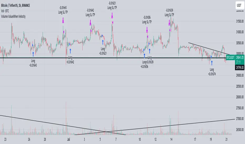
Volume ValueWhen VelocityTitle: Volume ValueWhen Velocity Trading Strategy
▶ Introduction:
The " Volume ValueWhen Velocity " trading strategy is designed to generate long position signals based on various technical conditions, including volume thresholds, RSI (Relative Strength Index), and price action relative to the Simple Moving Average (SMA). The strategy aims to identify potential buy opportunities when specific criteria are met, helping traders capitalize on potential bullish movements.
▶ How to use and conditions
★ Important : Only on Spot Binance BINANCE:BTCUSDT
Name: Volume ValueWhen Velocity
Operating mode: Long on Spot BINANCE BINANCE:BTCUSDT
Timeframe: Only one hour
Market: Crypto
currency: Bitcoin only
Signal type: Medium or short term
Entry: All sections in the Technical Indicators and Conditions section must be saved to enter (This is explained below)
Exit: Based on loss limit and profit limit It is removed in the settings section
Backtesting:
⁃ Exchange: BINANCE BINANCE:BTCUSDT
⁃ Pair: BTCUSDT
⁃ Timeframe:1h
⁃ Fee: 0.1%
- Initial Capital: 1,000 USDT
- Position sizing: 500 usdt
-Trading Range: 2022-07-01 11:30 ___ 2023-07-21 14:30
▶ Strategy Settings and Parameters:
1. `strategy(title='Volume ValueWhen Velocity', ...`: Sets the strategy title, initial capital, default quantity type, default quantity value, commission value, and trading currency.
↬ Stop-Loss and Take-Profit Settings:
1. long_stoploss_value and long_stoploss_percentage : Define the stop-loss percentage for long positions.
2. long_takeprofit_value and long_takeprofit_percentage : Define the take-profit percentage for long positions.
↬ ValueWhen Occurrence Parameters:
1. occurrence_ValueWhen_1 and occurrence_ValueWhen_2 : Control the occurrences of value events.
2. `distance_value`: Specifies the minimum distance between occurrences of ValueWhen 1 and ValueWhen 2.
↬ RSI Settings:
1. rsi_over_sold and rsi_length : Define the oversold level and RSI length for RSI calculations.
↬ Volume Thresholds:
1. volume_threshold1 , volume_threshold2 , and volume_threshold3 : Set the volume thresholds for multiple volume conditions.
↬ ATR (Average True Range) Settings:
1. atr_small and atr_big : Specify the periods used to calculate the Average True Range.
▶ Date Range for Back-Testing:
1. start_date, end_date, start_month, end_month, start_year, and end_year : Define the date range for back-testing the strategy.
▶ Technical Indicators and Conditions:
1. rsi: Calculates the Relative Strength Index (RSI) based on the defined RSI length and the closing prices.
2. was_over_sold: Checks if the RSI was oversold in the last 10 bars.
3. getVolume and getVolume2 : Custom functions to retrieve volume data for specific bars.
4. firstCandleColor : Evaluates the color of the first candle based on different timeframes.
5. sma : Calculates the Simple Moving Average (SMA) of the closing price over 13 periods.
6. numCandles : Counts the number of candles since the close price crossed above the SMA.
7. atr1 : Checks if the ATR_small is less than ATR_big for the specified security and timeframe.
8. prevClose, prevCloseBarsAgo, and prevCloseChange : ValueWhen functions to calculate the change in the close price between specific occurrences.
9. atrval: A condition based on the ATR_value3.
▶ Buy Signal Condition:
Condition: A combination of multiple volume conditions.
buy_signal: The final buy signal condition that considers various technical conditions and their interactions.
▶ Long Strategy Execution:
1. The strategy will enter a long position (buy) when the buy_signal condition is met and within the specified date range.
2. A stop-loss and take-profit will be set for the long position to manage risk and potential profits.
▶ Conclusion:
The " Volume ValueWhen Velocity " trading strategy is designed to identify long position opportunities based on a combination of volume conditions, RSI, and price action. The strategy aims to capitalize on potential bullish movements and utilizes a stop-loss and take-profit mechanism to manage risk and optimize potential returns. Traders can use this strategy as a starting point for their own trading systems or further customize it to suit their preferences and risk appetite. It is crucial to thoroughly back-test and validate any trading strategy before deploying it in live markets.
↯ Disclaimer:
Risk Management is crucial, so adjust stop loss to your comfort level. A tight stop loss can help minimise potential losses. Use at your own risk.
How you or we can improve? Source code is open so share your ideas!
Leave a comment and smash the boost button!
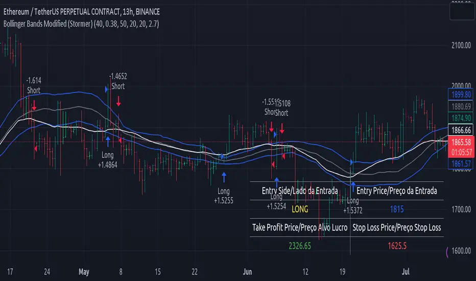
Bollinger Bands Modified (Stormer)This strategy is based and shown by trader and investor Alexandre Wolwacz "Stormer".
Overview
The strategy uses two indicators Bollinger Bands and EMA (optional for EMA).
Calculates Bollinger Bands, EMA, highest high, and lowest low values based on the input parameters, evaluating the conditions to determine potential long and short entry signals.
The conditions include checks for crossovers and crossunders of the price with the upper and lower Bollinger Bands, as well as the position of the price relative to the EMA.
The script also incorporates the option to add an inside bar pattern check for additional information.
Entry Position
Long Position:
Price cross over the superior band of bollinger bands.
The EMA is used to add support for trend analysis, it is an optional input, when used, it checks if price is above EMA.
Short Position:
Price cross under the inferior band of bollinger bands.
The EMA is used to add support for trend analysis, it is an optional input, when used, it checks if price is under EMA.
Risk Management
Stop Loss:
The stop loss is calculated based on the input highest high (for short position) and lowest low (for long position).
It gets the length based on the input from the last candles to set which is the highest high and which is the lowest low.
Take Profit:
According to the author, the profit target should be at least 1:1.6 the risk, so to have the strategy mathematically positive.
The profit target is configured input, can be increased or decreased.
It calculates the take profit based on the price of the stop loss with the profit target input.
Daily SPY PlanThe Daily SPY Plan indicator is a technical analysis tool designed to provide traders with a visual representation of price levels and take profit points for the SPY (S&P 500 ETF) on a daily timeframe. This indicator utilizes the Average True Range (ATR) to calculate projected price levels and take profit points, aiding traders in identifying potential breakout and profit-taking opportunities.
Indicator Description:
The indicator is written in Pine Script, specifically for use on the TradingView platform. It plots several levels on the price chart, each representing a potential breakout or take profit point. The levels are determined based on a fraction of the ATR added or subtracted from the closing price. The fractions used are 0.25, 0.5, 0.75, 1.0, 1.25, and 1.5 times the ATR.
The indicator distinguishes between breakout levels and take profit levels using different colors. Breakout levels, which indicate potential entry or exit points, are displayed in green, while take profit levels are shown in gray.
Key Features and Use:
ATR Calculation: The indicator calculates the Average True Range (ATR) using a specified length (default value of 14). ATR is a measure of market volatility and represents the average range between the high and low prices over a specific period.
Projected Price Levels: The indicator plots several projected price levels above and below the closing price. These levels are calculated by adding or subtracting a fraction of the ATR from the closing price. Traders can use these levels as potential breakout points or areas to set stop-loss orders.
Take Profit Points: The indicator also plots take profit points at specific levels above and below the closing price. These levels are designed to help traders identify potential areas to secure profits or partially exit their positions.
Visual Representation: The indicator utilizes step-like lines to plot the projected price levels and take profit points, providing a clear visual representation on the price chart. Traders can easily identify the relevant levels and incorporate them into their trading strategies.
Customizability: The indicator allows traders to customize the ATR length and choose whether to display Fibonacci levels (although there are no Fibonacci calculations in the provided code). These customization options enable traders to adapt the indicator to their preferred trading style and timeframe.
Limitations and Considerations:
Complementary Analysis: The Daily SPY Plan indicator should be used as a complementary tool alongside other technical analysis techniques and indicators. It provides price levels and take profit points based on ATR calculations, but it doesn't incorporate additional market factors or trading strategies.
Timeframe Suitability: The indicator is specifically designed for the daily timeframe of the SPY. Traders should consider adjusting the parameters and adapting the indicator if using it on different timeframes or instruments.
Risk Management: While the indicator suggests potential breakout and take profit points, it does not provide explicit stop-loss levels or risk management parameters. Traders should incorporate appropriate risk management techniques to protect their capital.
Conclusion:
The Daily SPY Plan indicator is a valuable technical analysis tool for traders focusing on the SPY ETF and the daily timeframe. By utilizing the ATR, it helps traders identify potential breakout levels and take profit points. However, traders should remember that this indicator is just one piece of the puzzle and should be used in conjunction with other technical analysis tools and risk management strategies to make informed trading decisions.

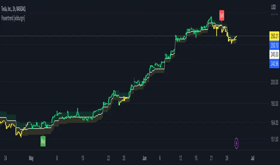
Powertrend - Volume Range Filter Strategy [wbburgin]The Powertrend is a range filter that is based off of volume, instead of price. This helps the range filter capture trends more accurately than a price-based range filter, because the range filter will update itself from changes in volume instead of changes in price. In certain scenarios this means that the Powertrend will be more profitable than a normal range filter.
Essentials of the Strategy
This is a breakout strategy which works best on trending assets with high volume and liquidity. It should be used on middle to higher timeframes and can be used on all assets that have volume provided by the data source (stocks, crypto, forex). It is long-only as of now. It can work on lower timeframes if you optimize the strategy filters to make less trades or if your exchange/broker is low/no fees, provided that your exchange/broker has high liquidity and volume.
The strategy enters a long position if the range filter is trending upwards and the price crosses over the upper range band, which signifies a price-volume breakout. The strategy closes the long position if the range filter is trending downwards and the price crosses under the lower range band, which signifies a breakdown. Both these conditions can be altered by the three filter options in the settings. The default trend filter is not alterable because it helps prevent false entries and exits that are against the trend.
Settings
The Length setting is the lookback period for the range smoothing.
The ADX Filter setting enables you to turn on an ADX filter, which will halt entries and exits unless the ADX of your customizable length is above a ADX VWMA of that length.
The Range Supertrend setting creates a supertrend from the top and bottom ranges, which can be used to filter entries and exits. The length is customizable. The filter can show you whether the range is making higher highs and lower lows. Below is an example of the Range Supertrend being used as a filter and plotted on-chart:
The VWMA setting halts entries if they are below a customizable length VWMA.
Both the Range Supertrend and the VWMA can also be plotted separately without actually filtering the strategy, so that you can use them independently if you wish. You can turn off the bar color, the highlighting, and the labels if you wish in the settings. A note about the bar color: if the color changes but the strategy does not signal an exit or entry this means that the crossover was against the trend. In these circumstances it may be indicative of a pullback to enter or exit or to add onto your position.
About the Strategy Results Below
A range filter is normally composed of two components - the range filter itself and a smoothing function. In the development of this script I tested both normal and volume-based varieties of the range filter and the smoothing function:
Tests Performed
Volume-based Range x VWMA smoothing
Price-based Range x VWMA smoothing
Price-based Range x EMA smoothing
Volume-based Range x EMA smoothing (final result)
The highest-performing was a volume-based range filter and a normal EMA-based smoothing function, but that does not mean that this strategy will be profitable - exits are based off of signal reversion so I strongly encourage you to develop your own take profits/stop losses for the strategy if you think it may be a good fit for you. The results below are with a commission value of 0.05% (because I built the strategy first for equities), slippage of 3, so if your exchange/broker has a higher fee schedule, I recommend adding filters and/or moving to higher timeframes for the strategy. Additionally, I used 10% of equity in each trade, while using the Range Supertrend filter (the previous upload was unrealistic because it used 100% of equity - missed a 0, apologies, and added in slippage).
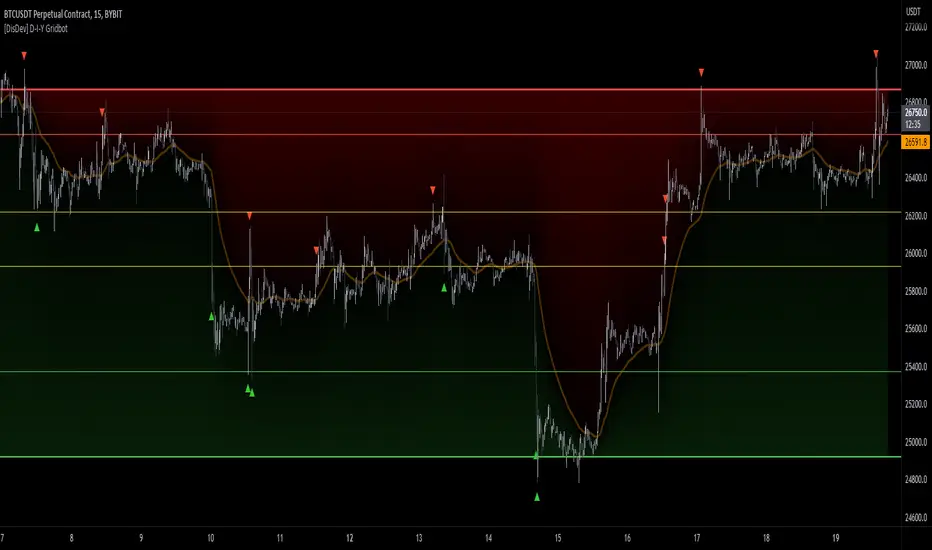
[DisDev] D-I-Y Gridbot🟩 This script is a “do-it-yourself” Grid Bot Simulator, used for visualizing support and resistance levels. Prices are divided into grids, or trade zones, that will trigger signals each time a new zone is entered. During ranging markets, each transaction is followed by a “take profit.” As the market starts to trend, transactions are stacked (compare to DCA ), until the market consolidates. No signals are triggered above the upper gridline or below the lower gridline. Unlike the previous version, all grids may be adjusted in real-time by dragging the gridlines up and down to the desired support and resistance levels.
When adding the indicator to a new chart, you must choose six grid levels by clicking on the desired support or resistance price. You can change all of these levels at any time directly on the chart.
⚡ OVERVIEW ⚡
The D-I-Y Gridbot is an interactive tool designed for visualizing support and resistance levels. As a continuation of the original Gridbot Simulator , which has received significant recognition on TradingView, earning over 4000 boosts and an Editor's Pick status. This tool serves not only as an evolved version of its predecessor, but also as an open-source template for developing future gridbots. It aims to foster discussions and facilitate innovations around grid-trading strategies.
One of the new features of this gridbot is the real-time adjustability of all gridlines. Users can move these lines up and down to set their desired support and resistance levels in response to changing market conditions. Additionally, the D-I-Y Gridbot is compatible with multiple timeframes and can be used on most TradingView charts.
Drag gridlines up or down to desired price level.
Key Features 🔑
All gridlines are adjustable in real-time, directly on the chart
Signals can be filtered by a customizable moving average or by VWAP
Customizable support and resistance levels
Potentially increases profitability in ranging markets
Benefits 💸
Customizable Support and Resistance Levels : The D-I-Y Gridbot allows users to set their preferred support and resistance levels, which can be changed at any time directly on the chart. This provides users with the ability to customize their trading parameters based on their strategy and risk tolerance.
Various Trading Strategies : The D-I-Y Gridbot supports various trading strategies, including Mean Reversion, Ranging Markets, and Dollar-cost averaging (DCA). This allows users to capitalize on price reversals, execute buy and sell orders at predetermined levels, and buy more of an asset as the price falls, respectively.
Multi-Timeframe and Versatility : The D-I-Y Gridbot is compatible with multiple timeframes and can be used on any TradingView chart.
Experimental and Educational : The D-I-Y Gridbot is considered a proof-of-concept tool that is both experimental and educational. This can provide traders with a deeper understanding of grid trading strategies and the ability to experiment with different trading parameters and strategies.
⚙️ CONFIGURATION & SETTINGS ⚙️
Inputs 🔧
Trigger : Candle location to trigger the signal. "Wick" will use either high or low, depending on the signal direction. "Close" will use the close price. “MA” will use the selected moving average or VWAP.
Confirmation : Market direction to confirm the candle trigger. "Reverse" will confirm the signal when the price crosses back over the trigger. "Breakout" will confirm when the price breaks out of the trigger.
Number of Support/Resistance zones : 1 = Only Top Grid is Support/Only Bottom Grid is Resistance. 2 = Top two grids are Resistance/Bottom two grids are Support. 3 = Top three grids are Resistance/Bottom three grids are Support
MA Type : Exponential Moving Average (EMA), Hull Moving Average (HMA), Simple Moving Average (SMA), Triple Exponential Moving Average (TEMA), Volume Weighted Moving Average (VWMA), Volume Weighted Average Price (VWAP)
MA Filter : Use Moving Average as a reversion filter for signals. When enabled, no buys when above MA, no sells when below. Use in conjunction with S/R zones to reduce false signals.
Allow Repeat Signals . When enabled, signals will reset when nearest gridline is triggered. When disabled, only one signal will be triggered per gridline.
Line/Fill colors
Gridlines . Adjusts gridline prices manually.
Left : Trigger = Wick. Confirm = Breakout. Buys are signaled when LOW breaks below gridline. Sells are triggered when HIGH breaks above gridline.
Right : Trigger = Close. Confirm = Breakout. Buys are signaled when the candle CLOSES below the gridline. Sells are triggered when the candle CLOSES above the gridline.
Left : Confirm=Breakout. Signals on breaking through the next gridline.
Right : Confirm=Reverse. Signals only when crossing back from the gridline.
S/R Zones=1. Upper gridline is Resistance / Lower is Support. Middle 4 are neutral.
S/R Zones = 3. Upper three gridlines are Resistance / Lower three are Support
Notes:
If gridlines are dragged out of order on a live chart, they will auto-sort into the correct order.
Price levels may be entered in settings, or adjusted in real-time directly on the chart.
When changing symbols, remember to adjust the gridlines to accommodate the new symbol.
Alerts 🔔
Users can set alerts based on their chosen parameters for triggers, confirmations, number of support/resistance zones, and smoothing type, enabling precise control over alert conditions.
💡 USAGE & STRATEGY 💡
Trading Strategies 📈
Mean Reversion: The script can be used to capitalize on price reversals back to the mean.
Ranging Markets: The script excels in ranging markets, executing buy and sell orders at predetermined levels.
Dollar-cost averaging (DCA): The script can be used to execute DCA orders, buying more of an asset as the price falls, and lowering the average cost per unit.
Timeframes and Symbols ⌚
Multi-Timeframe: The indicator is compatible with multiple timeframes.
Versatile: Can be used on any crypto trading pair on TradingView.
🤖 DETAILS & METHODOLOGY 🤖
Algorithm and Calculation 🛡️
Grids are set and adjusted when loading the indicator on the chart and may be customized anytime afterward by clicking and dragging the gridlines on the chart.
Gridlines are updated, sorted, and stored in a float array.
Signals are calculated based on candle trigger, market direction, and previous price level.
📚 ADDITIONAL RESOURCES 📚
Chart Examples 📊
S/R Zones = 3: Three Support and Three Resistance. Filter = 50-period Triple Exponential Moving Average (TEMA)
S/R Zones = 1: One Support, One Resistance, and Four Neutral Zones. Support Zones: Buys only. Resistance Zones: Sells only. Neutral Zones: Grid-dependent
When MA filter is enabled, Buys are only triggered below Moving Average, and Sells are only triggered above.
Trigger = Wick. Confirmation = Breakout. Buys are signaled when Low breaks above the next grid level. Sells are signaled when High breaks below the next grid level.
🚀 CONCLUSION 🚀
The D-I-Y Gridbot is a proof-of-concept, emphasizing its experimental and educational nature. In future versions, we will aim to incorporate concepts such as auto-adjusting grids and angled grids for trending markets. The script is designed to evolve through user feedback and suggestions, shaping its future iterations.
Credit: This is a continuation of the Gridbot series by xxattaxx-DisDev . Explicit permission was granted by user xxattaxx-disdev to re-use all Gridbot code and all materials without restrictions.
⚠️ DISCLAIMER ⚠️
This indicator is a proof-of-concept and is considered experimental and educational. When gridlines are drawn in hindsight, signals appear to be predictive and valid. Future results may always vary when the trend direction changes. Comments and suggestions are encouraged.
This indicator is provided as a tool for traders and should not be used as the sole basis for making trading decisions. Always conduct your own research and consider your risk tolerance before entering any trades.
D-Bot Alpha RSI Breakout StrategyHello dear Traders,
Here is a simple yet effective strategy to use, for best profit higher time frame, such as daily.
Structure of the code
The code defines inputs for SMA (simple moving average) length, RSI (relative strength index) length, RSI entry level, RSI stop loss level, and RSI take profit level. The default values of these variables can be customized as per the user's preferences.
The script calculates SMA and RSI based on the input parameters and the closing price of the asset.
Trading logic
This strategy allows the placement of a long position when:
The RSI crosses above the RSI entry level and
The close price is above the SMA value.
After entering a long position, it applies a trailing stop mechanism. The stop price is updated to the close price if the close price is lower than the last close price.
The script closes the long position when:
RSI falls below the stop loss level.
RSI reaches or exceeds the take profit level.
If the trailing stop is activated (once RSI reaches or exceeds the take profit level), the closing price falls below the trailing stop level.
Strengths
The strategy includes mechanisms for entering a position, taking profit, and stopping losses, which are fundamental aspects of a trading strategy.
It applies a trailing stop mechanism that allows to capture further gains if the price keeps increasing while protecting from losses if the price starts to decrease.
Weaknesses
This strategy only contemplates long positions. Depending on the market situation, the strategy may miss opportunities for short selling when the market is on a downward trend.
The choice of the fixed RSI entry, stop loss, and take profit levels may not be ideal for all market conditions or assets. It might benefit from a more adaptive mechanism that adjusts these levels according to market volatility or trend.
The strategy doesn't factor in trading costs (such as spread or commission), which could have a significant impact on the net profit, especially if the user is trading with a high frequency or in a low liquidity market.
How to trade with this strategy
Given these parameters and the strategy outlined by the code, the trader would enter a long position when the RSI crosses above the RSI entry level (default 34) and the closing price is above the SMA value (SMA calculated with default period of 200). The trader would exit the position when either the RSI falls below the RSI stop loss level (default 30), or RSI rises above the RSI take profit level (default 50), or when the trailing stop is hit.
Remember "The strategies I have prepared are entirely for educational purposes and should not be considered as investment advice. Support your trades using other tools. Wishing everyone profitable trades..."

Mechanical Trading StrategyThe "Mechanical Trading Strategy" is a simple and systematic approach to trading that aims to capture short-term price movements in the financial markets. This strategy focuses on executing trades based on specific conditions and predetermined profit targets and stop loss levels.
Key Features:
Profit Target: The strategy allows you to set a profit target as a percentage of the entry price. This target represents the desired level of profit for each trade.
Stop Loss: The strategy incorporates a stop loss level as a percentage of the entry price. This level represents the maximum acceptable loss for each trade, helping to manage risk.
Entry Condition: The strategy triggers trades at a specific time. In this case, the condition for entering a trade is based on the hour of the candle being 16 (4:00 PM). This time-based entry condition provides a systematic approach to executing trades.
Position Sizing: The strategy determines the position size based on a fixed percentage of the available equity. This approach ensures consistent risk management and allows for potential portfolio diversification.
Execution:
When the entry condition is met, signified by the hour being 16, the strategy initiates a long position using the strategy.entry function. It sets the exit conditions using the strategy.exit function, with a limit order for the take profit level and a stop order for the stop loss level.
Take Profit and Stop Loss:
The take profit level is calculated by adding a percentage of the entry price to the entry price itself. This represents the profit target for the trade. Conversely, the stop loss level is calculated by subtracting a percentage of the entry price from the entry price. This level represents the maximum acceptable loss for the trade.
By using this mechanical trading strategy, traders can establish a disciplined and systematic approach to their trading decisions. The predefined profit target and stop loss levels provide clear exit rules, helping to manage risk and potentially maximize returns. However, it is important to note that no trading strategy is guaranteed to be profitable, and careful analysis and monitoring of market conditions are always recommended.

Alpha Fractal BandsWilliams fractals are remarkable support and resistance levels used by many traders. However, it can sometimes be challenging to use them frequently and get confirmation from other oscillators and indicators. With the new "Alpha Fractal Bands", a unique blend of Williams Fractals and Bollinger Bands emerges, offering a fresh perspective. Extremes can be utilized as price reversals or for taking profits. I look forward to hearing your thoughts. Best regards... Happy trading!
An easy solution for long positions is to:
Identify a bullish trend or a potential entry point for a long position.
Set a stop-loss order to limit potential losses if the trade goes against you.
Determine a target price or take-profit level to lock in profits.
Consider using technical indicators or analysis tools to confirm the strength of the bullish trend.
Regularly monitor the trade and make necessary adjustments based on market conditions.
An easy solution for short positions could be to follow these steps:
Identify a bearish trend or a potential entry point for a short position.
Set a stop-loss order to limit potential losses if the trade goes against you.
Determine a target price or take-profit level to lock in profits.
Consider using technical indicators or analysis tools to confirm the strength of the bearish trend.
Regularly monitor the trade and make necessary adjustments based on market conditions.
Remember, it's important to conduct thorough research and analysis before entering any trade and to manage your risk effectively.
To stay updated with the content, don't forget to follow and engage with it on TV, my friends. Remember to leave comments as well :)

VWAP Trendfollow Strategy [wbburgin]This is an experimental strategy that enters long when the instrument crosses over the upper standard deviation band of a VWAP and enters short when the instrument crosses below the bottom standard deviation band of the VWAP. I have added a trend filter as well, which stops entries that are opposite to the current trend of the VWAP. The trend filter will reduce total false breakouts, thus improving the % profitable while maintaining the overall returns of the strategy. Because this is a trend-following breakout strategy, the % profitable will typically be low but the average % return will be higher. As a rule, be sure to look at the average winning trade % compared to the average losing trade %, and compare that to the % profitable to judge the effectiveness of a strategy. Factor in fees and slippage as well.
This strategy appears to work better with the lower timeframes, and I was impressed with its results. It also appears to work on a wide range of asset classes. There isn't a stop loss or take profit built-in (other than the reversal signals, which close the current trade), so I would encourage you to expand on the strategy based on your own trading parameters.
You can toggle off the bar colors and the trend filter if you so desire.
Future updates to this script (or ideas of improving on it) might include a take profit level set at one standard deviation past the current level and a stop loss level set at one standard deviation closer to the vwap from the current level - or applying a multiple to the two based off of your reward/risk ratio.
About the strategy results below: this is with commissions of 0.5 % per trade.

Inside candle (Inside Bar) Strategy- by smartanuThe Inside Candle strategy is a popular price action trading strategy that can be used to trade in a variety of markets. Here's how you can trade the Inside Candle strategy using the Pine script code provided:
1. Identify an Inside Candle: Look for a candlestick pattern where the current candle is completely engulfed within the previous candle's high and low. This is known as an Inside Candle.
2. Enter a Long Position: If an Inside Candle is identified, enter a long position at the open of the next candle using the Pine script code provided.
3. Set Stop Loss and Take Profit: Set a stop loss at a reasonable level to limit your potential losses if the trade goes against you. Set a take profit at a reasonable level to take profit when the price reaches the desired level.
4. Manage the Trade: Monitor the trade closely and adjust the stop loss and take profit levels if necessary. You can use the Pine script code to automatically exit the trade when the stop loss or take profit level is hit.
5. Exit the Trade: Exit the trade when the price reaches the take profit level or the stop loss level is hit.
It's important to note that the Inside Candle strategy is just one of many strategies that traders use to trade the markets. It's important to perform your own analysis and use additional indicators before making any trades. Additionally, it's important to practice proper risk management techniques and never risk more than you can afford to lose.

Goertzel Cycle Composite Wave [Loxx]As the financial markets become increasingly complex and data-driven, traders and analysts must leverage powerful tools to gain insights and make informed decisions. One such tool is the Goertzel Cycle Composite Wave indicator, a sophisticated technical analysis indicator that helps identify cyclical patterns in financial data. This powerful tool is capable of detecting cyclical patterns in financial data, helping traders to make better predictions and optimize their trading strategies. With its unique combination of mathematical algorithms and advanced charting capabilities, this indicator has the potential to revolutionize the way we approach financial modeling and trading.
*** To decrease the load time of this indicator, only XX many bars back will render to the chart. You can control this value with the setting "Number of Bars to Render". This doesn't have anything to do with repainting or the indicator being endpointed***
█ Brief Overview of the Goertzel Cycle Composite Wave
The Goertzel Cycle Composite Wave is a sophisticated technical analysis tool that utilizes the Goertzel algorithm to analyze and visualize cyclical components within a financial time series. By identifying these cycles and their characteristics, the indicator aims to provide valuable insights into the market's underlying price movements, which could potentially be used for making informed trading decisions.
The Goertzel Cycle Composite Wave is considered a non-repainting and endpointed indicator. This means that once a value has been calculated for a specific bar, that value will not change in subsequent bars, and the indicator is designed to have a clear start and end point. This is an important characteristic for indicators used in technical analysis, as it allows traders to make informed decisions based on historical data without the risk of hindsight bias or future changes in the indicator's values. This means traders can use this indicator trading purposes.
The repainting version of this indicator with forecasting, cycle selection/elimination options, and data output table can be found here:
Goertzel Browser
The primary purpose of this indicator is to:
1. Detect and analyze the dominant cycles present in the price data.
2. Reconstruct and visualize the composite wave based on the detected cycles.
To achieve this, the indicator performs several tasks:
1. Detrending the price data: The indicator preprocesses the price data using various detrending techniques, such as Hodrick-Prescott filters, zero-lag moving averages, and linear regression, to remove the underlying trend and focus on the cyclical components.
2. Applying the Goertzel algorithm: The indicator applies the Goertzel algorithm to the detrended price data, identifying the dominant cycles and their characteristics, such as amplitude, phase, and cycle strength.
3. Constructing the composite wave: The indicator reconstructs the composite wave by combining the detected cycles, either by using a user-defined list of cycles or by selecting the top N cycles based on their amplitude or cycle strength.
4. Visualizing the composite wave: The indicator plots the composite wave, using solid lines for the cycles. The color of the lines indicates whether the wave is increasing or decreasing.
This indicator is a powerful tool that employs the Goertzel algorithm to analyze and visualize the cyclical components within a financial time series. By providing insights into the underlying price movements, the indicator aims to assist traders in making more informed decisions.
█ What is the Goertzel Algorithm?
The Goertzel algorithm, named after Gerald Goertzel, is a digital signal processing technique that is used to efficiently compute individual terms of the Discrete Fourier Transform (DFT). It was first introduced in 1958, and since then, it has found various applications in the fields of engineering, mathematics, and physics.
The Goertzel algorithm is primarily used to detect specific frequency components within a digital signal, making it particularly useful in applications where only a few frequency components are of interest. The algorithm is computationally efficient, as it requires fewer calculations than the Fast Fourier Transform (FFT) when detecting a small number of frequency components. This efficiency makes the Goertzel algorithm a popular choice in applications such as:
1. Telecommunications: The Goertzel algorithm is used for decoding Dual-Tone Multi-Frequency (DTMF) signals, which are the tones generated when pressing buttons on a telephone keypad. By identifying specific frequency components, the algorithm can accurately determine which button has been pressed.
2. Audio processing: The algorithm can be used to detect specific pitches or harmonics in an audio signal, making it useful in applications like pitch detection and tuning musical instruments.
3. Vibration analysis: In the field of mechanical engineering, the Goertzel algorithm can be applied to analyze vibrations in rotating machinery, helping to identify faulty components or signs of wear.
4. Power system analysis: The algorithm can be used to measure harmonic content in power systems, allowing engineers to assess power quality and detect potential issues.
The Goertzel algorithm is used in these applications because it offers several advantages over other methods, such as the FFT:
1. Computational efficiency: The Goertzel algorithm requires fewer calculations when detecting a small number of frequency components, making it more computationally efficient than the FFT in these cases.
2. Real-time analysis: The algorithm can be implemented in a streaming fashion, allowing for real-time analysis of signals, which is crucial in applications like telecommunications and audio processing.
3. Memory efficiency: The Goertzel algorithm requires less memory than the FFT, as it only computes the frequency components of interest.
4. Precision: The algorithm is less susceptible to numerical errors compared to the FFT, ensuring more accurate results in applications where precision is essential.
The Goertzel algorithm is an efficient digital signal processing technique that is primarily used to detect specific frequency components within a signal. Its computational efficiency, real-time capabilities, and precision make it an attractive choice for various applications, including telecommunications, audio processing, vibration analysis, and power system analysis. The algorithm has been widely adopted since its introduction in 1958 and continues to be an essential tool in the fields of engineering, mathematics, and physics.
█ Goertzel Algorithm in Quantitative Finance: In-Depth Analysis and Applications
The Goertzel algorithm, initially designed for signal processing in telecommunications, has gained significant traction in the financial industry due to its efficient frequency detection capabilities. In quantitative finance, the Goertzel algorithm has been utilized for uncovering hidden market cycles, developing data-driven trading strategies, and optimizing risk management. This section delves deeper into the applications of the Goertzel algorithm in finance, particularly within the context of quantitative trading and analysis.
Unveiling Hidden Market Cycles:
Market cycles are prevalent in financial markets and arise from various factors, such as economic conditions, investor psychology, and market participant behavior. The Goertzel algorithm's ability to detect and isolate specific frequencies in price data helps trader analysts identify hidden market cycles that may otherwise go unnoticed. By examining the amplitude, phase, and periodicity of each cycle, traders can better understand the underlying market structure and dynamics, enabling them to develop more informed and effective trading strategies.
Developing Quantitative Trading Strategies:
The Goertzel algorithm's versatility allows traders to incorporate its insights into a wide range of trading strategies. By identifying the dominant market cycles in a financial instrument's price data, traders can create data-driven strategies that capitalize on the cyclical nature of markets.
For instance, a trader may develop a mean-reversion strategy that takes advantage of the identified cycles. By establishing positions when the price deviates from the predicted cycle, the trader can profit from the subsequent reversion to the cycle's mean. Similarly, a momentum-based strategy could be designed to exploit the persistence of a dominant cycle by entering positions that align with the cycle's direction.
Enhancing Risk Management:
The Goertzel algorithm plays a vital role in risk management for quantitative strategies. By analyzing the cyclical components of a financial instrument's price data, traders can gain insights into the potential risks associated with their trading strategies.
By monitoring the amplitude and phase of dominant cycles, a trader can detect changes in market dynamics that may pose risks to their positions. For example, a sudden increase in amplitude may indicate heightened volatility, prompting the trader to adjust position sizing or employ hedging techniques to protect their portfolio. Additionally, changes in phase alignment could signal a potential shift in market sentiment, necessitating adjustments to the trading strategy.
Expanding Quantitative Toolkits:
Traders can augment the Goertzel algorithm's insights by combining it with other quantitative techniques, creating a more comprehensive and sophisticated analysis framework. For example, machine learning algorithms, such as neural networks or support vector machines, could be trained on features extracted from the Goertzel algorithm to predict future price movements more accurately.
Furthermore, the Goertzel algorithm can be integrated with other technical analysis tools, such as moving averages or oscillators, to enhance their effectiveness. By applying these tools to the identified cycles, traders can generate more robust and reliable trading signals.
The Goertzel algorithm offers invaluable benefits to quantitative finance practitioners by uncovering hidden market cycles, aiding in the development of data-driven trading strategies, and improving risk management. By leveraging the insights provided by the Goertzel algorithm and integrating it with other quantitative techniques, traders can gain a deeper understanding of market dynamics and devise more effective trading strategies.
█ Indicator Inputs
src: This is the source data for the analysis, typically the closing price of the financial instrument.
detrendornot: This input determines the method used for detrending the source data. Detrending is the process of removing the underlying trend from the data to focus on the cyclical components.
The available options are:
hpsmthdt: Detrend using Hodrick-Prescott filter centered moving average.
zlagsmthdt: Detrend using zero-lag moving average centered moving average.
logZlagRegression: Detrend using logarithmic zero-lag linear regression.
hpsmth: Detrend using Hodrick-Prescott filter.
zlagsmth: Detrend using zero-lag moving average.
DT_HPper1 and DT_HPper2: These inputs define the period range for the Hodrick-Prescott filter centered moving average when detrendornot is set to hpsmthdt.
DT_ZLper1 and DT_ZLper2: These inputs define the period range for the zero-lag moving average centered moving average when detrendornot is set to zlagsmthdt.
DT_RegZLsmoothPer: This input defines the period for the zero-lag moving average used in logarithmic zero-lag linear regression when detrendornot is set to logZlagRegression.
HPsmoothPer: This input defines the period for the Hodrick-Prescott filter when detrendornot is set to hpsmth.
ZLMAsmoothPer: This input defines the period for the zero-lag moving average when detrendornot is set to zlagsmth.
MaxPer: This input sets the maximum period for the Goertzel algorithm to search for cycles.
squaredAmp: This boolean input determines whether the amplitude should be squared in the Goertzel algorithm.
useAddition: This boolean input determines whether the Goertzel algorithm should use addition for combining the cycles.
useCosine: This boolean input determines whether the Goertzel algorithm should use cosine waves instead of sine waves.
UseCycleStrength: This boolean input determines whether the Goertzel algorithm should compute the cycle strength, which is a normalized measure of the cycle's amplitude.
WindowSizePast: These inputs define the window size for the composite wave.
FilterBartels: This boolean input determines whether Bartel's test should be applied to filter out non-significant cycles.
BartNoCycles: This input sets the number of cycles to be used in Bartel's test.
BartSmoothPer: This input sets the period for the moving average used in Bartel's test.
BartSigLimit: This input sets the significance limit for Bartel's test, below which cycles are considered insignificant.
SortBartels: This boolean input determines whether the cycles should be sorted by their Bartel's test results.
StartAtCycle: This input determines the starting index for selecting the top N cycles when UseCycleList is set to false. This allows you to skip a certain number of cycles from the top before selecting the desired number of cycles.
UseTopCycles: This input sets the number of top cycles to use for constructing the composite wave when UseCycleList is set to false. The cycles are ranked based on their amplitudes or cycle strengths, depending on the UseCycleStrength input.
SubtractNoise: This boolean input determines whether to subtract the noise (remaining cycles) from the composite wave. If set to true, the composite wave will only include the top N cycles specified by UseTopCycles.
█ Exploring Auxiliary Functions
The following functions demonstrate advanced techniques for analyzing financial markets, including zero-lag moving averages, Bartels probability, detrending, and Hodrick-Prescott filtering. This section examines each function in detail, explaining their purpose, methodology, and applications in finance. We will examine how each function contributes to the overall performance and effectiveness of the indicator and how they work together to create a powerful analytical tool.
Zero-Lag Moving Average:
The zero-lag moving average function is designed to minimize the lag typically associated with moving averages. This is achieved through a two-step weighted linear regression process that emphasizes more recent data points. The function calculates a linearly weighted moving average (LWMA) on the input data and then applies another LWMA on the result. By doing this, the function creates a moving average that closely follows the price action, reducing the lag and improving the responsiveness of the indicator.
The zero-lag moving average function is used in the indicator to provide a responsive, low-lag smoothing of the input data. This function helps reduce the noise and fluctuations in the data, making it easier to identify and analyze underlying trends and patterns. By minimizing the lag associated with traditional moving averages, this function allows the indicator to react more quickly to changes in market conditions, providing timely signals and improving the overall effectiveness of the indicator.
Bartels Probability:
The Bartels probability function calculates the probability of a given cycle being significant in a time series. It uses a mathematical test called the Bartels test to assess the significance of cycles detected in the data. The function calculates coefficients for each detected cycle and computes an average amplitude and an expected amplitude. By comparing these values, the Bartels probability is derived, indicating the likelihood of a cycle's significance. This information can help in identifying and analyzing dominant cycles in financial markets.
The Bartels probability function is incorporated into the indicator to assess the significance of detected cycles in the input data. By calculating the Bartels probability for each cycle, the indicator can prioritize the most significant cycles and focus on the market dynamics that are most relevant to the current trading environment. This function enhances the indicator's ability to identify dominant market cycles, improving its predictive power and aiding in the development of effective trading strategies.
Detrend Logarithmic Zero-Lag Regression:
The detrend logarithmic zero-lag regression function is used for detrending data while minimizing lag. It combines a zero-lag moving average with a linear regression detrending method. The function first calculates the zero-lag moving average of the logarithm of input data and then applies a linear regression to remove the trend. By detrending the data, the function isolates the cyclical components, making it easier to analyze and interpret the underlying market dynamics.
The detrend logarithmic zero-lag regression function is used in the indicator to isolate the cyclical components of the input data. By detrending the data, the function enables the indicator to focus on the cyclical movements in the market, making it easier to analyze and interpret market dynamics. This function is essential for identifying cyclical patterns and understanding the interactions between different market cycles, which can inform trading decisions and enhance overall market understanding.
Bartels Cycle Significance Test:
The Bartels cycle significance test is a function that combines the Bartels probability function and the detrend logarithmic zero-lag regression function to assess the significance of detected cycles. The function calculates the Bartels probability for each cycle and stores the results in an array. By analyzing the probability values, traders and analysts can identify the most significant cycles in the data, which can be used to develop trading strategies and improve market understanding.
The Bartels cycle significance test function is integrated into the indicator to provide a comprehensive analysis of the significance of detected cycles. By combining the Bartels probability function and the detrend logarithmic zero-lag regression function, this test evaluates the significance of each cycle and stores the results in an array. The indicator can then use this information to prioritize the most significant cycles and focus on the most relevant market dynamics. This function enhances the indicator's ability to identify and analyze dominant market cycles, providing valuable insights for trading and market analysis.
Hodrick-Prescott Filter:
The Hodrick-Prescott filter is a popular technique used to separate the trend and cyclical components of a time series. The function applies a smoothing parameter to the input data and calculates a smoothed series using a two-sided filter. This smoothed series represents the trend component, which can be subtracted from the original data to obtain the cyclical component. The Hodrick-Prescott filter is commonly used in economics and finance to analyze economic data and financial market trends.
The Hodrick-Prescott filter is incorporated into the indicator to separate the trend and cyclical components of the input data. By applying the filter to the data, the indicator can isolate the trend component, which can be used to analyze long-term market trends and inform trading decisions. Additionally, the cyclical component can be used to identify shorter-term market dynamics and provide insights into potential trading opportunities. The inclusion of the Hodrick-Prescott filter adds another layer of analysis to the indicator, making it more versatile and comprehensive.
Detrending Options: Detrend Centered Moving Average:
The detrend centered moving average function provides different detrending methods, including the Hodrick-Prescott filter and the zero-lag moving average, based on the selected detrending method. The function calculates two sets of smoothed values using the chosen method and subtracts one set from the other to obtain a detrended series. By offering multiple detrending options, this function allows traders and analysts to select the most appropriate method for their specific needs and preferences.
The detrend centered moving average function is integrated into the indicator to provide users with multiple detrending options, including the Hodrick-Prescott filter and the zero-lag moving average. By offering multiple detrending methods, the indicator allows users to customize the analysis to their specific needs and preferences, enhancing the indicator's overall utility and adaptability. This function ensures that the indicator can cater to a wide range of trading styles and objectives, making it a valuable tool for a diverse group of market participants.
The auxiliary functions functions discussed in this section demonstrate the power and versatility of mathematical techniques in analyzing financial markets. By understanding and implementing these functions, traders and analysts can gain valuable insights into market dynamics, improve their trading strategies, and make more informed decisions. The combination of zero-lag moving averages, Bartels probability, detrending methods, and the Hodrick-Prescott filter provides a comprehensive toolkit for analyzing and interpreting financial data. The integration of advanced functions in a financial indicator creates a powerful and versatile analytical tool that can provide valuable insights into financial markets. By combining the zero-lag moving average,
█ In-Depth Analysis of the Goertzel Cycle Composite Wave Code
The Goertzel Cycle Composite Wave code is an implementation of the Goertzel Algorithm, an efficient technique to perform spectral analysis on a signal. The code is designed to detect and analyze dominant cycles within a given financial market data set. This section will provide an extremely detailed explanation of the code, its structure, functions, and intended purpose.
Function signature and input parameters:
The Goertzel Cycle Composite Wave function accepts numerous input parameters for customization, including source data (src), the current bar (forBar), sample size (samplesize), period (per), squared amplitude flag (squaredAmp), addition flag (useAddition), cosine flag (useCosine), cycle strength flag (UseCycleStrength), past sizes (WindowSizePast), Bartels filter flag (FilterBartels), Bartels-related parameters (BartNoCycles, BartSmoothPer, BartSigLimit), sorting flag (SortBartels), and output buffers (goeWorkPast, cyclebuffer, amplitudebuffer, phasebuffer, cycleBartelsBuffer).
Initializing variables and arrays:
The code initializes several float arrays (goeWork1, goeWork2, goeWork3, goeWork4) with the same length as twice the period (2 * per). These arrays store intermediate results during the execution of the algorithm.
Preprocessing input data:
The input data (src) undergoes preprocessing to remove linear trends. This step enhances the algorithm's ability to focus on cyclical components in the data. The linear trend is calculated by finding the slope between the first and last values of the input data within the sample.
Iterative calculation of Goertzel coefficients:
The core of the Goertzel Cycle Composite Wave algorithm lies in the iterative calculation of Goertzel coefficients for each frequency bin. These coefficients represent the spectral content of the input data at different frequencies. The code iterates through the range of frequencies, calculating the Goertzel coefficients using a nested loop structure.
Cycle strength computation:
The code calculates the cycle strength based on the Goertzel coefficients. This is an optional step, controlled by the UseCycleStrength flag. The cycle strength provides information on the relative influence of each cycle on the data per bar, considering both amplitude and cycle length. The algorithm computes the cycle strength either by squaring the amplitude (controlled by squaredAmp flag) or using the actual amplitude values.
Phase calculation:
The Goertzel Cycle Composite Wave code computes the phase of each cycle, which represents the position of the cycle within the input data. The phase is calculated using the arctangent function (math.atan) based on the ratio of the imaginary and real components of the Goertzel coefficients.
Peak detection and cycle extraction:
The algorithm performs peak detection on the computed amplitudes or cycle strengths to identify dominant cycles. It stores the detected cycles in the cyclebuffer array, along with their corresponding amplitudes and phases in the amplitudebuffer and phasebuffer arrays, respectively.
Sorting cycles by amplitude or cycle strength:
The code sorts the detected cycles based on their amplitude or cycle strength in descending order. This allows the algorithm to prioritize cycles with the most significant impact on the input data.
Bartels cycle significance test:
If the FilterBartels flag is set, the code performs a Bartels cycle significance test on the detected cycles. This test determines the statistical significance of each cycle and filters out the insignificant cycles. The significant cycles are stored in the cycleBartelsBuffer array. If the SortBartels flag is set, the code sorts the significant cycles based on their Bartels significance values.
Waveform calculation:
The Goertzel Cycle Composite Wave code calculates the waveform of the significant cycles for specified time windows. The windows are defined by the WindowSizePast parameters, respectively. The algorithm uses either cosine or sine functions (controlled by the useCosine flag) to calculate the waveforms for each cycle. The useAddition flag determines whether the waveforms should be added or subtracted.
Storing waveforms in a matrix:
The calculated waveforms for the cycle is stored in the matrix - goeWorkPast. This matrix holds the waveforms for the specified time windows. Each row in the matrix represents a time window position, and each column corresponds to a cycle.
Returning the number of cycles:
The Goertzel Cycle Composite Wave function returns the total number of detected cycles (number_of_cycles) after processing the input data. This information can be used to further analyze the results or to visualize the detected cycles.
The Goertzel Cycle Composite Wave code is a comprehensive implementation of the Goertzel Algorithm, specifically designed for detecting and analyzing dominant cycles within financial market data. The code offers a high level of customization, allowing users to fine-tune the algorithm based on their specific needs. The Goertzel Cycle Composite Wave's combination of preprocessing, iterative calculations, cycle extraction, sorting, significance testing, and waveform calculation makes it a powerful tool for understanding cyclical components in financial data.
█ Generating and Visualizing Composite Waveform
The indicator calculates and visualizes the composite waveform for specified time windows based on the detected cycles. Here's a detailed explanation of this process:
Updating WindowSizePast:
The WindowSizePast is updated to ensure they are at least twice the MaxPer (maximum period).
Initializing matrices and arrays:
The matrix goeWorkPast is initialized to store the Goertzel results for specified time windows. Multiple arrays are also initialized to store cycle, amplitude, phase, and Bartels information.
Preparing the source data (srcVal) array:
The source data is copied into an array, srcVal, and detrended using one of the selected methods (hpsmthdt, zlagsmthdt, logZlagRegression, hpsmth, or zlagsmth).
Goertzel function call:
The Goertzel function is called to analyze the detrended source data and extract cycle information. The output, number_of_cycles, contains the number of detected cycles.
Initializing arrays for waveforms:
The goertzel array is initialized to store the endpoint Goertzel.
Calculating composite waveform (goertzel array):
The composite waveform is calculated by summing the selected cycles (either from the user-defined cycle list or the top cycles) and optionally subtracting the noise component.
Drawing composite waveform (pvlines):
The composite waveform is drawn on the chart using solid lines. The color of the lines is determined by the direction of the waveform (green for upward, red for downward).
To summarize, this indicator generates a composite waveform based on the detected cycles in the financial data. It calculates the composite waveforms and visualizes them on the chart using colored lines.
█ Enhancing the Goertzel Algorithm-Based Script for Financial Modeling and Trading
The Goertzel algorithm-based script for detecting dominant cycles in financial data is a powerful tool for financial modeling and trading. It provides valuable insights into the past behavior of these cycles. However, as with any algorithm, there is always room for improvement. This section discusses potential enhancements to the existing script to make it even more robust and versatile for financial modeling, general trading, advanced trading, and high-frequency finance trading.
Enhancements for Financial Modeling
Data preprocessing: One way to improve the script's performance for financial modeling is to introduce more advanced data preprocessing techniques. This could include removing outliers, handling missing data, and normalizing the data to ensure consistent and accurate results.
Additional detrending and smoothing methods: Incorporating more sophisticated detrending and smoothing techniques, such as wavelet transform or empirical mode decomposition, can help improve the script's ability to accurately identify cycles and trends in the data.
Machine learning integration: Integrating machine learning techniques, such as artificial neural networks or support vector machines, can help enhance the script's predictive capabilities, leading to more accurate financial models.
Enhancements for General and Advanced Trading
Customizable indicator integration: Allowing users to integrate their own technical indicators can help improve the script's effectiveness for both general and advanced trading. By enabling the combination of the dominant cycle information with other technical analysis tools, traders can develop more comprehensive trading strategies.
Risk management and position sizing: Incorporating risk management and position sizing functionality into the script can help traders better manage their trades and control potential losses. This can be achieved by calculating the optimal position size based on the user's risk tolerance and account size.
Multi-timeframe analysis: Enhancing the script to perform multi-timeframe analysis can provide traders with a more holistic view of market trends and cycles. By identifying dominant cycles on different timeframes, traders can gain insights into the potential confluence of cycles and make better-informed trading decisions.
Enhancements for High-Frequency Finance Trading
Algorithm optimization: To ensure the script's suitability for high-frequency finance trading, optimizing the algorithm for faster execution is crucial. This can be achieved by employing efficient data structures and refining the calculation methods to minimize computational complexity.
Real-time data streaming: Integrating real-time data streaming capabilities into the script can help high-frequency traders react to market changes more quickly. By continuously updating the cycle information based on real-time market data, traders can adapt their strategies accordingly and capitalize on short-term market fluctuations.
Order execution and trade management: To fully leverage the script's capabilities for high-frequency trading, implementing functionality for automated order execution and trade management is essential. This can include features such as stop-loss and take-profit orders, trailing stops, and automated trade exit strategies.
While the existing Goertzel algorithm-based script is a valuable tool for detecting dominant cycles in financial data, there are several potential enhancements that can make it even more powerful for financial modeling, general trading, advanced trading, and high-frequency finance trading. By incorporating these improvements, the script can become a more versatile and effective tool for traders and financial analysts alike.
█ Understanding the Limitations of the Goertzel Algorithm
While the Goertzel algorithm-based script for detecting dominant cycles in financial data provides valuable insights, it is important to be aware of its limitations and drawbacks. Some of the key drawbacks of this indicator are:
Lagging nature:
As with many other technical indicators, the Goertzel algorithm-based script can suffer from lagging effects, meaning that it may not immediately react to real-time market changes. This lag can lead to late entries and exits, potentially resulting in reduced profitability or increased losses.
Parameter sensitivity:
The performance of the script can be sensitive to the chosen parameters, such as the detrending methods, smoothing techniques, and cycle detection settings. Improper parameter selection may lead to inaccurate cycle detection or increased false signals, which can negatively impact trading performance.
Complexity:
The Goertzel algorithm itself is relatively complex, making it difficult for novice traders or those unfamiliar with the concept of cycle analysis to fully understand and effectively utilize the script. This complexity can also make it challenging to optimize the script for specific trading styles or market conditions.
Overfitting risk:
As with any data-driven approach, there is a risk of overfitting when using the Goertzel algorithm-based script. Overfitting occurs when a model becomes too specific to the historical data it was trained on, leading to poor performance on new, unseen data. This can result in misleading signals and reduced trading performance.
Limited applicability:
The Goertzel algorithm-based script may not be suitable for all markets, trading styles, or timeframes. Its effectiveness in detecting cycles may be limited in certain market conditions, such as during periods of extreme volatility or low liquidity.
While the Goertzel algorithm-based script offers valuable insights into dominant cycles in financial data, it is essential to consider its drawbacks and limitations when incorporating it into a trading strategy. Traders should always use the script in conjunction with other technical and fundamental analysis tools, as well as proper risk management, to make well-informed trading decisions.
█ Interpreting Results
The Goertzel Cycle Composite Wave indicator can be interpreted by analyzing the plotted lines. The indicator plots two lines: composite waves. The composite wave represents the composite wave of the price data.
The composite wave line displays a solid line, with green indicating a bullish trend and red indicating a bearish trend.
Interpreting the Goertzel Cycle Composite Wave indicator involves identifying the trend of the composite wave lines and matching them with the corresponding bullish or bearish color.
█ Conclusion
The Goertzel Cycle Composite Wave indicator is a powerful tool for identifying and analyzing cyclical patterns in financial markets. Its ability to detect multiple cycles of varying frequencies and strengths make it a valuable addition to any trader's technical analysis toolkit. However, it is important to keep in mind that the Goertzel Cycle Composite Wave indicator should be used in conjunction with other technical analysis tools and fundamental analysis to achieve the best results. With continued refinement and development, the Goertzel Cycle Composite Wave indicator has the potential to become a highly effective tool for financial modeling, general trading, advanced trading, and high-frequency finance trading. Its accuracy and versatility make it a promising candidate for further research and development.
█ Footnotes
What is the Bartels Test for Cycle Significance?
The Bartels Cycle Significance Test is a statistical method that determines whether the peaks and troughs of a time series are statistically significant. The test is named after its inventor, George Bartels, who developed it in the mid-20th century.
The Bartels test is designed to analyze the cyclical components of a time series, which can help traders and analysts identify trends and cycles in financial markets. The test calculates a Bartels statistic, which measures the degree of non-randomness or autocorrelation in the time series.
The Bartels statistic is calculated by first splitting the time series into two halves and calculating the range of the peaks and troughs in each half. The test then compares these ranges using a t-test, which measures the significance of the difference between the two ranges.
If the Bartels statistic is greater than a critical value, it indicates that the peaks and troughs in the time series are non-random and that there is a significant cyclical component to the data. Conversely, if the Bartels statistic is less than the critical value, it suggests that the peaks and troughs are random and that there is no significant cyclical component.
The Bartels Cycle Significance Test is particularly useful in financial analysis because it can help traders and analysts identify significant cycles in asset prices, which can in turn inform investment decisions. However, it is important to note that the test is not perfect and can produce false signals in certain situations, particularly in noisy or volatile markets. Therefore, it is always recommended to use the test in conjunction with other technical and fundamental indicators to confirm trends and cycles.
Deep-dive into the Hodrick-Prescott Fitler
The Hodrick-Prescott (HP) filter is a statistical tool used in economics and finance to separate a time series into two components: a trend component and a cyclical component. It is a powerful tool for identifying long-term trends in economic and financial data and is widely used by economists, central banks, and financial institutions around the world.
The HP filter was first introduced in the 1990s by economists Robert Hodrick and Edward Prescott. It is a simple, two-parameter filter that separates a time series into a trend component and a cyclical component. The trend component represents the long-term behavior of the data, while the cyclical component captures the shorter-term fluctuations around the trend.
The HP filter works by minimizing the following objective function:
Minimize: (Sum of Squared Deviations) + λ (Sum of Squared Second Differences)
Where:
1. The first term represents the deviation of the data from the trend.
2. The second term represents the smoothness of the trend.
3. λ is a smoothing parameter that determines the degree of smoothness of the trend.
The smoothing parameter λ is typically set to a value between 100 and 1600, depending on the frequency of the data. Higher values of λ lead to a smoother trend, while lower values lead to a more volatile trend.
The HP filter has several advantages over other smoothing techniques. It is a non-parametric method, meaning that it does not make any assumptions about the underlying distribution of the data. It also allows for easy comparison of trends across different time series and can be used with data of any frequency.
However, the HP filter also has some limitations. It assumes that the trend is a smooth function, which may not be the case in some situations. It can also be sensitive to changes in the smoothing parameter λ, which may result in different trends for the same data. Additionally, the filter may produce unrealistic trends for very short time series.
Despite these limitations, the HP filter remains a valuable tool for analyzing economic and financial data. It is widely used by central banks and financial institutions to monitor long-term trends in the economy, and it can be used to identify turning points in the business cycle. The filter can also be used to analyze asset prices, exchange rates, and other financial variables.
The Hodrick-Prescott filter is a powerful tool for analyzing economic and financial data. It separates a time series into a trend component and a cyclical component, allowing for easy identification of long-term trends and turning points in the business cycle. While it has some limitations, it remains a valuable tool for economists, central banks, and financial institutions around the world.

Cycle Position TradingTitle: Cycle Position Trading Strategy v1.0
Description: Cycle Position Trading Strategy is a simple yet effective trading strategy based on a 200-day Simple Moving Average (SMA). Users can select between two modes, "Buy Uptrend" and "Buy Downtrend," to customize the strategy according to their trading preferences. The strategy allows users to set their own stop loss (SL) and take profit (TP) levels, providing more flexibility and control over their trades.
Features:
Choose between two trading modes: "Buy Uptrend" and "Buy Downtrend."
Customize your stop loss (SL) and take profit (TP) levels.
Clear visual representation of the 200-day Simple Moving Average (SMA) on the chart.
How to use:
Add the strategy to your chart by searching for "Cycle Position Trading Strategy" in the TradingView "Indicators & Strategies" section.
Configure the strategy settings according to your preferences:
Select the trading mode from the dropdown menu. "Buy Uptrend" will open long positions when the closing price is above the 200-day SMA. "Buy Downtrend" will open long positions when the closing price is below the 200-day SMA.
Set your desired stop loss (SL) and take profit (TP) levels. The default values are 0.9 (10% below the entry price) for the stop loss and 1.1 (10% above the entry price) for the take profit.
Monitor the chart for trade signals based on the chosen mode and settings. The strategy will enter and exit trades automatically based on the selected mode and the configured stop loss and take profit levels.
Analyze the performance of the strategy by checking the TradingView strategy performance summary or by viewing individual trades in the "Trades" list.
Disclaimer: This strategy is intended for educational and illustrative purposes only. Use it at your own risk. Past performance is not indicative of future results. Trading stocks, cryptocurrencies, or any other financial instrument involves significant risk and may result in the loss of capital.
Version: v1.0
Release date: 2023-03-25
Author: I11L
License: Mozilla Public License 2.0 (mozilla.org)

Strategy for UT Bot Alerts indicator Using the UT Bot alerts indicator by @QuantNomad, this strategy was designed for showing an example of how this indicator could be used, also, it has the goal to help some people from a group that use to use this indicator for their trading. Under any circumstance I recommend to use it without testing it before in real time.
Backtesting context: 2020-02-05 to 2023-02-25 of BTCUSD 4H by Tvc. Commissions: 0.03% for each entry, 0.03% for each exit. Risk per trade: 2.5% of the total account
For this strategy, 3 indicators are used:
UT Bot Alerts indicator by Quantnomad
One Ema of 200 periods for indicate the trend
Atr stop loss from Gatherio
Trade conditions:
For longs:
Close price is higher than Atr from UT Bot
Ema from UT Bot cross over Atr from UT Bot.
This gives us our long signal. Stop loss will be determined by atr stop loss (white point), break even(blue point) by a risk/reward ratio of 0.75:1 and take profit of 3:1 where half position will be closed. This will be showed as buy (open long position)
The other half will be closed when close price is lower than Atr and Ema from UT Bot cross under Atr. This will be showed as cl buy (close long position)
For shorts:
Close price is lower than Atr from UT Bot
Ema from UT Bot cross over Atr from UT Bot.
This gives us our short signal. Stop loss will be determined by atr stop loss (white point), break even(blue point) by a risk/reward ratio of 0.75:1 and take profit of 3:1 where half position will be closed. This will be showed as sell (open short position)
The other half will be closed when close price is higher than Atr and Ema from UT Bot cross over Atr. This will be showed as cl sell (close short position)
Risk management
For calculate the amount of the position you will use just a small percent of your initial capital for the strategy and you will use the atr stop loss for this.
Example: You have 1000 usd and you just want to risk 2,5% of your account, there is a long signal at price of 20,000 usd. The stop loss price from atr stop loss is 19,000. You calculate the distance in percent between 20,000 and 19,000. In this case, that distance would be of 5,0%. Then, you calculate your position by this way: (initial or current capital * risk per trade of your account) / (stop loss distance).
Using these values on the formula: (1000*2,5%)/(5,0%) = 500usd. It means, you have to use 500 usd for risking 2.5% of your account.
We will use this risk management for apply compound interest.
In settings, with position amount calculator, you can enter the amount in usd of your account and the amount in percentage for risking per trade of the account. You will see this value in green color in the upper left corner that shows the amount in usd to use for risking the specific percentage of your account.
Script functions
Inside of settings, you will find some utilities for display atr stop loss, break evens, positions, signals, indicators, etc.
You will find the settings for risk management at the end of the script if you want to change something. But rebember, do not change values from indicators, the idea is to not over optimize the strategy.
If you want to change the initial capital for backtest the strategy, go to properties, and also enter the commisions of your exchange and slippage for more realistic results.
In risk managment you can find an option called "Use leverage ?", activate this if you want to backtest using leverage, which means that in case of not having enough money for risking the % determined by you of your account using your initial capital, you will use leverage for using the enough amount for risking that % of your acount in a buy position. Otherwise, the amount will be limited by your initial/current capital
---> Do not forget to deactivate Trades on chart option in style settings for a cleaner look of the chart <---
Some things to consider
USE UNDER YOUR OWN RISK. PAST RESULTS DO NOT REPRESENT THE FUTURE.
DEPENDING OF % ACCOUNT RISK PER TRADE, YOU COULD REQUIRE LEVERAGE FOR OPEN SOME POSITIONS, SO PLEASE, BE CAREFULL AND USE CORRECTLY THE RISK MANAGEMENT
Do not forget to change commissions and other parameters related with back testing results!
Strategies for trending markets use to have more looses than wins and it takes a long time to get profits, so do not forget to be patient and consistent !
---> The strategy can still be improved, you can change some parameters depending of the asset and timeframe like risk/reward for taking profits, for break even, also the main parameters of the UT Bot Alerts <----
Ema ScalpThis is another simple strategy based on ema
Entry Buy - 1) when close crossover ema then buy and only open one trade till it not close
2) if previous buy trade is profitable open another trade and check again trade is profitable or not
3)if trade is not profitable reset and wait for sell condition...
Entry Sell -1) when close crossunder ema then sell and only open one trade till it not close
2) if previous sell trade is profitable open another trade and check again trade is profitable or not
3) if trade is not profitable reset and wait for buy condition.....
stop loss and take profit is percentage based ...
